Examine This Report on Sumif Excel

By pushing ctrl+shift+facility, this will certainly determine and return value from multiple ranges, as opposed to simply specific cells included to or increased by one another. Computing the sum, product, or ratio of specific cells is simple-- just use the =AMOUNT formula and go into the cells, values, or series of cells you want to execute that arithmetic on.

If you're seeking to locate total sales revenue from several marketed devices, for instance, the variety formula in Excel is perfect for you. Right here's exactly how you would certainly do it: To begin making use of the range formula, type "=SUM," and also in parentheses, go into the very first of 2 (or three, or four) series of cells you 'd like to increase with each other.

This represents multiplication. Following this asterisk, enter your 2nd variety of cells. You'll be multiplying this 2nd variety of cells by the initial. Your progression in this formula should now appear like this: =AMOUNT(C 2: C 5 * D 2:D 5) Ready to push Get in? Not so quick ... Due to the fact that this formula is so challenging, Excel books a various key-board command for ranges.

This will recognize your formula as a selection, wrapping your formula in brace characters as well as successfully returning your product of both arrays incorporated. In earnings calculations, this can reduce your effort and time significantly. See the final formula in the screenshot over. The COUNT formula in Excel is denoted =MATTER(Start Cell: End Cell).

As an example, if there are 8 cells with entered worths between A 1 and also A 10, =MATTER(A 1: A 10) will return a value of 8. The COUNT formula in Excel is specifically beneficial for huge spread sheets, where you intend to see exactly how numerous cells consist of actual entries. Don't be misleaded: This formula won't do any mathematics on the values of the cells themselves.

The Best Guide To Excel Jobs

Utilizing the formula in vibrant above, you can conveniently run a matter of active cells in your spreadsheet. The result will look a something like this: To carry out the average formula in Excel, go into the values, cells, or variety of cells of which you're calculating the average in the style, =STANDARD(number 1, number 2, and so on) or =AVERAGE(Begin Worth: End Worth).

Locating the standard of a series of cells in Excel keeps you from needing to find specific amounts and also after that executing a separate department equation on your overall. Making use of =AVERAGE as your initial message entry, you can let Excel do all the benefit you. For recommendation, the standard of a team of numbers is equal to the amount of those numbers, divided by the variety of things because group.

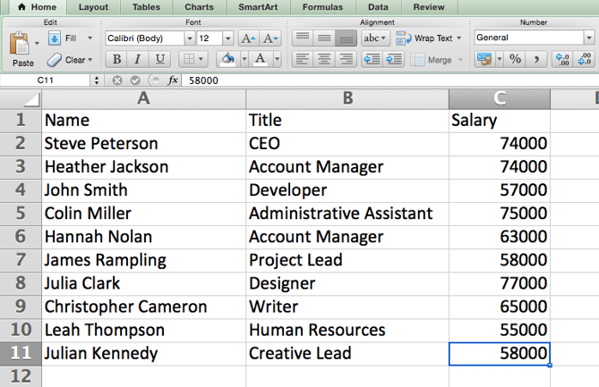
This will return the amount of the values within a desired series of cells that all fulfill one criterion. For instance, =SUMIF(C 3: C 12,"> 70,000") would certainly return the amount of values between cells C 3 and C 12 from just the cells that are more than 70,000. Allow's state you intend to determine the earnings you produced from a list of leads that are related to particular area codes, or determine the sum of specific employees' incomes-- however just if they fall above a certain amount.

With the SUMIF function, it does not have to be-- you can easily add up the sum of cells that fulfill particular criteria, like in the salary example above. The formula: =SUMIF(array, criteria, [sum_range] Range: The range that is being examined utilizing your standards. Standards: The standards that determine which cells in Criteria_range 1 will certainly be totaled [Sum_range]: An optional array of cells you're going to accumulate along with the very first Array went into.

In the example below, we desired to determine the amount of the incomes that were above $70,000. The SUMIF feature built up the buck quantities that surpassed that number in the cells C 3 through C 12, with the formula =SUMIF(C 3: C 12,"> 70,000"). The TRIM formula in Excel is denoted =TRIM(message).

The Main Principles Of Excel If Formula

As an example, if A 2 consists of the name" Steve Peterson" with undesirable areas prior to the given name, =TRIM(A 2) would certainly return "Steve Peterson" without spaces in a new cell. Email as well as submit sharing are terrific devices in today's work environment. That is, until among your coworkers sends you a worksheet with some truly cool spacing.

Rather than painstakingly removing and adding rooms as needed, you can cleanse up any uneven spacing using the TRIM feature, which is made use of to get rid of additional spaces from information (besides solitary spaces between words). The formula: =TRIM(message). Text: The message or cell where you intend to remove spaces.

To do so, we went into =TRIM("A 2") into the Solution Bar, and reproduced this for each and every name listed below it in a new column alongside the column with unwanted areas. Below are a few other Excel formulas you could discover valuable as your information management requires expand. Let's claim you have a line of message within a cell that you intend to damage down into a couple of various segments.

Objective: Utilized to extract the very first X numbers or personalities in a cell. The formula: =LEFT(message, number_of_characters) Text: The string that you desire to remove from. Number_of_characters: The number of personalities that you wish to extract beginning with the left-most personality. In the example below, we entered =LEFT(A 2,4) into cell B 2, as well as duplicated it into B 3: B 6.

Purpose: Used to extract characters or numbers between based on setting. The formula: =MID(text, start_position, number_of_characters) Text: The string that you wish to draw out from. Start_position: The position in the string that you desire to start extracting from. For example, the very first placement in the string is 1.

Getting My Excel If Formula To Work

In this instance, we went into =MID(A 2,5,2) right into cell B 2, and duplicated it right into B 3: B 6. That permitted us to remove both numbers beginning in the fifth position of the code. Objective: Made use of to remove the last X numbers or personalities in a cell. The formula: =RIGHT(message, number_of_characters) Text: The string that you wish to draw out from.

formulas excel basicas formulas excel en espanol formula excel if cell is not blank